"Every search method has a blind spot. A hybrid is not a bigger algorithm — it is one method placed exactly where another cannot see."- Claude 2026
Hybrid Optimization Techniques
No single search method is good at everything. Some roam widely but finish sloppily; some polish an answer beautifully but never leave the neighborhood they started in. Hybrid optimization is the deliberate practice of bolting one method onto another so that each covers the other's blind spot.
Optimization means searching a space of possible solutions for the one that scores best under some measure — shortest route, lowest cost, highest yield. A heuristic is a rule of thumb that finds good answers without guaranteeing the best; a metaheuristic is a general strategy for steering such rules, like evolution or swarming. This page assumes no background in any of them: each idea is described plainly before it is named.
Learning objectives
By the end of this page you should be able to:
- Define the concept of hybrid optimization and identify its components.
- Design a hybrid optimization model by integrating multiple AI techniques.
- Evaluate the advantages and limitations of hybrid optimization approaches.
Why Hybridize at All?
Picture the set of all possible answers to a problem as a landscape, where height is cost and you are looking for the lowest point. A smooth landscape has one valley: walk downhill and you are done. A rugged one is pitted with thousands of dips, and downhill walking traps you in whichever dip you happened to start near.
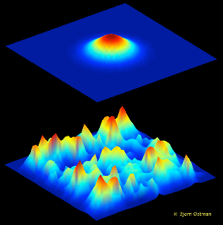
Real optimization problems are rugged, and that ruggedness splits search methods into two temperaments. Exploration means covering ground: sampling far-apart regions so you notice a valley you were not standing in. Exploitation means squeezing the region you already have: small careful adjustments that drive the score down as far as it will go. Every algorithm strikes some balance, and no algorithm strikes a good one everywhere.
Here is the same story as a picture. A global method takes long, undirected jumps; a local method takes short, strictly downhill steps. Alone, either wastes effort. Alternated, they cover the landscape and then mine each promising spot properly.
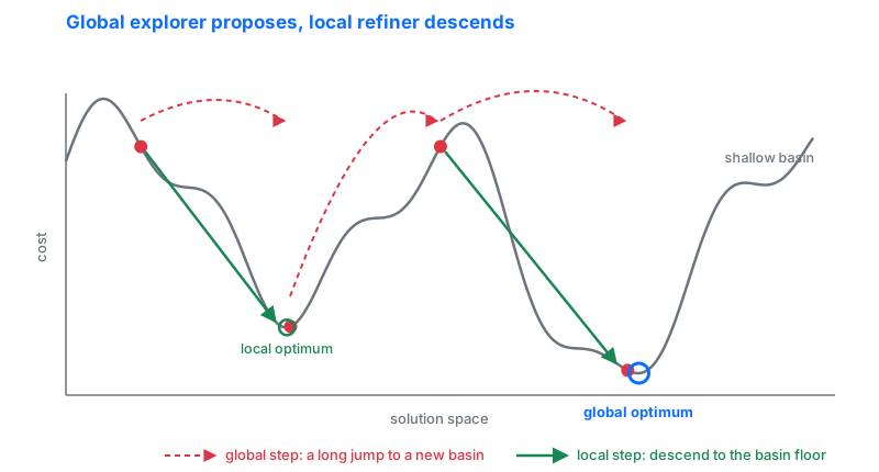
Framed this way, the families of methods you might combine each have an obvious strength and an equally obvious weakness:
| Component | Good at | Blind spot |
|---|---|---|
| Evolutionary algorithms | Broad exploration; recombining partial solutions; no gradient required | Slow, imprecise endgame — rarely nails the last few percent |
| Swarm methods | Fast coverage of continuous spaces; trivially parallel | Premature convergence once the swarm clumps together |
| Local search | Rapid, reliable improvement from any starting point | Stops at the first local optimum it reaches |
| Exact solvers (LP, MILP, CP) | Provable optimality; hard constraints handled natively | Blows up on large instances; needs a formal model |
| Machine learning and RL | Learning patterns across many similar instances | Needs data or training time; offers no guarantees |
| Surrogate models | Standing in for an evaluation that costs hours or dollars | Only as good as its approximation; misleads if wrong |
Anatomy of a Hybrid
Strip away the naming and almost every hybrid has the same three slots. Not all three are always filled, but knowing which slot a component occupies tells you what it is there to do.
Filling those slots with different materials gives the recognized families of hybrid method. The names below are the ones you will meet in the literature.
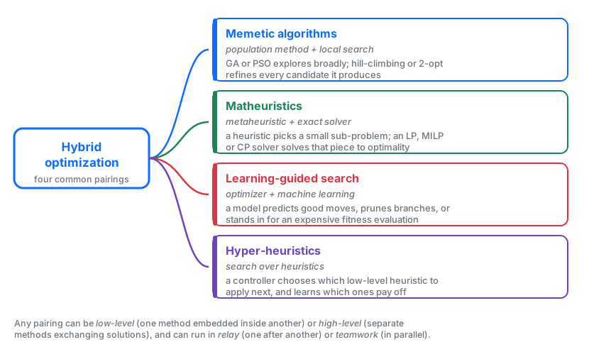
Memetic algorithms
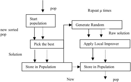
The classic hybrid: run an evolutionary algorithm, but before evaluating any individual, run a local search on it first. Evolution supplies variety across the whole population; local search makes sure each individual is judged at its best rather than at whatever half-finished state mutation left it in. The name comes from Dawkins' "meme" — the idea that individuals improve within their lifetime, not only across generations.
Matheuristics
Exact solvers give provably optimal answers but choke on large instances. A matheuristic keeps the solver and shrinks the problem: fix most of the current solution, free a small slice of it, and let the solver optimize that slice exactly. Repeat with a different slice. This is the idea behind large neighborhood search, which powers much industrial routing and scheduling software.
Large neighborhood search, in four steps
- Start from any feasible solution.
- Destroy: remove part of it — say 15% of customers from a set of delivery routes.
- Repair: hand the fragment to an exact solver, which re-inserts those customers optimally.
- Accept if improved, then destroy a different part. The neighborhood searched each round is enormous, but the solver only ever sees a small problem.
Learning-guided search
Here the third slot gets filled. A model trained on past instances predicts which branches of a search tree to expand, which crossover to apply, or which candidates deserve a full evaluation. The most established version is surrogate-assisted optimization: when each evaluation costs a wind-tunnel run or a week of simulation, fit a cheap statistical model of the objective, search that, and spend real evaluations only where the model is either promising or uncertain. Bayesian optimization is this idea with the uncertainty handled formally.
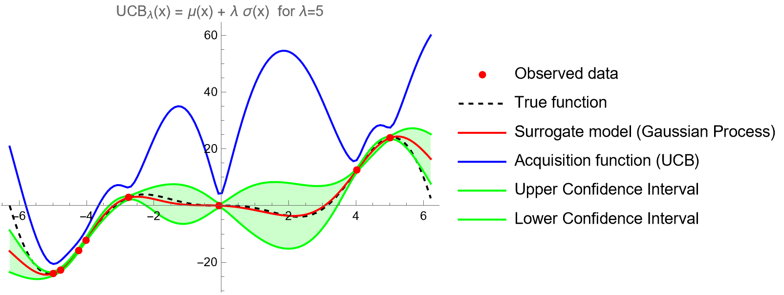
Hyper-heuristics take the guide idea one level up: rather than searching for a solution, the controller searches for a method, choosing at each step which low-level heuristic to apply and learning from the reward which ones tend to pay off. When that controller is a reinforcement learning agent, the boundary between "optimization" and "learning" essentially disappears.
Designing a Hybrid
Hybridizing is not "use more algorithms". The useful discipline is to name the specific failure you are compensating for before you add anything.
The example below follows that recipe on a 60-city travelling salesman problem. The explorer is a small genetic algorithm with order crossover; the refiner is 2-opt, which repeatedly reverses a segment of the tour whenever doing so shortens it. A single flag switches the refiner off, so the hybrid can be measured against its own explorer:
import random
import math

random.seed(7)
cities = [(random.uniform(0, 100), random.uniform(0, 100)) for _ in range(60)]

def dist(a, b):
    return math.dist(cities[a], cities[b])

def tour_length(t):
    return sum(dist(t[i], t[i - 1]) for i in range(len(t)))

def two_opt(t):
    n, improved = len(t), True
    while improved:
        improved = False
        for i in range(1, n - 1):
            for j in range(i + 1, n):
                a, b, c, d = t[i - 1], t[i], t[j], t[(j + 1) % n]
                if dist(a, b) + dist(c, d) > dist(a, c) + dist(b, d):
                    t[i:j + 1] = reversed(t[i:j + 1])
                    improved = True
    return t

def order_crossover(p1, p2):
    n = len(p1)
    i, j = sorted(random.sample(range(n), 2))
    child = [None] * n
    child[i:j] = p1[i:j]
    fill = (c for c in p2 if c not in set(p1[i:j]))
    return [c if c is not None else next(fill) for c in child]

def mutate(t, rate=0.2):
    if random.random() < rate:
        i, j = sorted(random.sample(range(len(t)), 2))
        t[i:j] = reversed(t[i:j])
    return t

def evolve(pop_size=40, generations=60, memetic=True):
    pop = [random.sample(range(len(cities)), len(cities)) for _ in range(pop_size)]
    if memetic:
        pop = [two_opt(t) for t in pop]
    for _ in range(generations):
        pop.sort(key=tour_length)
        elite = pop[:pop_size // 4]
        children = []
        while len(children) < pop_size - len(elite):
            p1, p2 = random.sample(elite, 2)
            child = mutate(order_crossover(p1, p2))
            children.append(two_opt(child) if memetic else child)
        pop = elite + children
    return min(pop, key=tour_length)

print('plain GA  ', round(tour_length(evolve(memetic=False))))
print('memetic GA', round(tour_length(evolve(memetic=True))))
That gap is typical, and it is worth being honest about where it comes from: most of the improvement here is 2-opt, not evolution. The evolutionary layer earns its keep on harder instances by recombining different locally-optimal tours into a better one — something 2-opt alone cannot do, because it never leaves the basin it starts in.
The same pattern in continuous space needs no bespoke code at all. SciPy's basin-hopping is a two-component hybrid in the plainest possible form: random jumps as the explorer, a gradient-based minimizer as the refiner. On the Rastrigin function — a lattice of local minima around one global minimum at the origin — the difference is the whole point of this page:
import numpy as np
from scipy.optimize import basinhopping, minimize

def rastrigin(x):
    return 10 * len(x) + np.sum(x ** 2 - 10 * np.cos(2 * np.pi * x))

x0 = np.array([4.2, -3.7])
local = minimize(rastrigin, x0)
hybrid = basinhopping(rastrigin, x0, niter=200, seed=0,
                      minimizer_kwargs={'method': 'L-BFGS-B'})
print('local only', round(local.fun, 4), local.x.round(3))
print('hybrid    ', round(hybrid.fun, 4), hybrid.x.round(3))
The local minimizer alone returns 31.84 at [3.98, -3.98] — the bottom of whichever pit it started in. Adding the hopping layer returns 0.0 at the origin. Nothing about the refiner changed; it simply got asked the question from better starting points.
Advantages and Limitations
Hybrids dominate the leaderboards of most optimization competitions, and they are the standard architecture in industrial routing, scheduling, and design software. That success is real, but it is not free.
- Better solutions per unit time. The refiner turns rough candidates into competitive ones, so the explorer's budget is spent comparing real answers.
- Fewer expensive evaluations. A surrogate or learned guide can cut simulation-heavy workloads by orders of magnitude.
- Robustness across instances. Where a single method is brittle to problem structure, a hybrid degrades gracefully.
- Constraints handled properly. Pairing a heuristic with an exact solver keeps hard constraints satisfied by construction rather than by penalty terms.
- Anytime behavior. Most hybrids hold a feasible incumbent from early on, so you can stop whenever the deadline arrives.
- Parameter explosion. Two methods bring two parameter sets plus the ones governing their interaction, and tuning cost grows combinatorially.
- Cost per iteration. A memetic generation can cost fifty times a plain one; compared on iterations rather than seconds, hybrids flatter themselves.
- Diversity collapse. Aggressive local search drags the population into the same basins, quietly turning a global search into a local one.
- Lost guarantees. Wrapping an exact solver in a heuristic loop discards its optimality proof — you get speed, not certainty.
- Complexity and reproducibility. More moving parts means more places to hide a bug, and published hybrids are notoriously hard to reproduce.
- Benchmark overfitting. A hybrid tuned on one instance family often loses to a simple method on the next one.
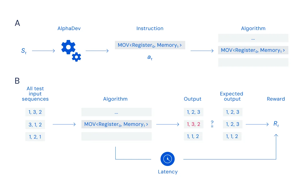
The most compelling recent evidence for the approach comes from systems where a learned guide steers a classical search. AlphaDev searched the space of assembly instruction sequences with a reinforcement learning agent playing what was framed as a single-player game, and found sorting routines faster than the human-written ones that had stood in the C++ standard library for over a decade.
Tools & Tutorials
- SciPy basinhopping and dual_annealing — two ready-made global-plus-local hybrids with runnable examples; the fastest way to feel the difference the refiner makes.
- pymoo — a Python framework whose algorithms accept custom repair, local-search, and initialization operators, making memetic variants a few lines of code.
- pygmo 2 — the "island model": several different optimizers run in parallel and periodically migrate solutions to one another, which is high-level teamwork hybridization out of the box.
- Mealpy — around 200 population-based optimizers behind one interface, useful for comparing candidate explorers before committing to a pairing.
- Optuna's CMA-ES sampler — a practical surrogate-and-search hybrid for tuning; note the documented pattern of starting with random or TPE sampling and switching to CMA-ES once enough trials exist.
- Nevergrad — gradient-free optimization whose default recommendation is a portfolio that picks and blends methods based on problem dimension and budget: hyper-heuristics as a library default.
- NEOS Optimization Guide — a concise map of the exact-solver side of the field, worth skimming before pairing a heuristic with an LP, MILP, or CP model.
Further reading
- Neri, F., Cotta, C. & Moscato, P. (eds.) (2012). Handbook of Memetic Algorithms. — the standard reference on population methods coupled with local search, including how much refinement to apply and to whom.
- Vanaret, C. (2020). Hybridization of Interval Methods and Evolutionary Algorithms for Solving Difficult Optimization Problems. — its opening chapters give an unusually clear, freely readable account of hybridization taxonomies before diving into the author's own method.
- Bello, I. et al. (2017). Neural Combinatorial Optimization with Reinforcement Learning. — the paper that made learned guides for combinatorial search a mainstream research direction.
- Dai, H. et al. (2017). Learning Combinatorial Optimization Algorithms over Graphs. — a graph network learns a greedy construction heuristic, a concrete and readable instance of the guide-plus-explorer pattern.
- Mirhoseini, A. et al. (2021). A Graph Placement Methodology for Fast Chip Design. Nature. — reinforcement learning paired with classical placement optimization on a problem where hours of expert work were the baseline.