"A Q-table has one cell per situation. The moment "situation" means a screen of pixels, the table is larger than the universe — so you stop storing values and start predicting them."- Claude 2026
Advanced Reinforcement Learning Techniques
Tabular methods learn one value per state and work beautifully — until the states run out. Real problems have too many situations to ever list, so modern reinforcement learning replaces the table with a neural network and, from there, opens up a whole family of far more capable algorithms.
In reinforcement learning an agent takes actions in an environment and learns from a scalar reward, aiming to maximize its long-run return. Classic Q-learning stores an estimated value for every state–action pair in a lookup table. This page picks up where that leaves off: what to do when the table can't fit, how learning the policy directly changes the game, and how these methods hold up in messy, moving-target environments. No prior deep-learning detail is assumed — each idea is introduced plainly before the formal name.
Learning objectives
By the end of this page you should be able to:
- Describe advanced reinforcement learning methods such as deep reinforcement learning.
- Compare policy-gradient and actor-critic methods with traditional reinforcement learning.
- Evaluate the performance of advanced reinforcement learning in dynamic environments.
Deep Reinforcement Learning
A Q-table needs one row per state. That is fine for a 4×4 gridworld, but consider an Atari game: the state is the screen, and the number of possible screens is astronomically larger than the number of atoms in the universe. You could never visit them all, let alone store a value for each. The fix is to stop memorizing values and start predicting them.
Wiring a neural network into Q-learning is the Deep Q-Network (DQN), the method that first learned to play dozens of Atari games from raw pixels at human level. Pixels flow through convolutional layers; the network outputs one Q-value per possible action; the agent picks the largest.
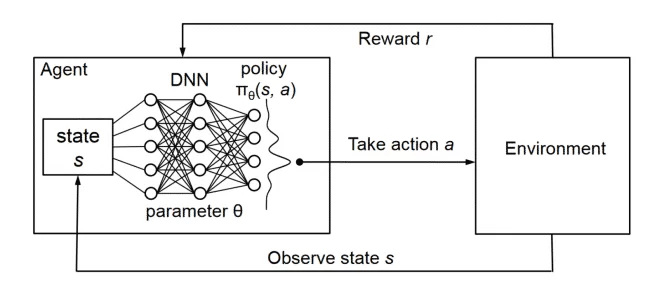
Naively training this network is unstable, because consecutive frames are highly correlated and the target the network chases keeps shifting. Two ideas make it work, and they appear in nearly every deep-RL method since:
In code, the DQN loss is just the tabular Q-update rewritten as a regression problem — predicted value versus reward-plus-discounted-best-next, with the target computed by the frozen copy:
import torch
import torch.nn as nn

def dqn_loss(q_net, target_net, s, a, r, s_next, done, gamma=0.99):
    q_sa = q_net(s).gather(1, a.unsqueeze(1)).squeeze(1)
    with torch.no_grad():
        best_next = target_net(s_next).max(1).values
        target = r + gamma * best_next * (1 - done)
    return nn.functional.mse_loss(q_sa, target)
Everything downstream — Double DQN, Dueling DQN, Rainbow — refines this same skeleton. But DQN still only estimates values and then acts greedily. A different and often more powerful idea is to skip the value estimate and learn the behavior itself.
Policy Gradients and Actor-Critic vs. Traditional RL
Traditional (value-based) RL learns "how good is each action?" and then picks the best. Policy-gradient methods take a more direct route: they represent the policy itself as a network πθ(a|s) and adjust its parameters to make high-reward actions more likely. There is no table of values in between — you optimize the behavior directly.
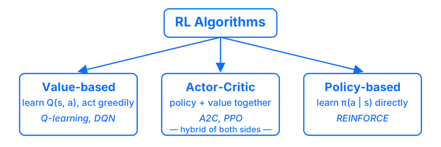
The simplest policy-gradient algorithm is REINFORCE: run an episode, then push up the probability of every action taken in proportion to the return that followed it. Good episodes reinforce their actions; bad ones suppress theirs.
import torch

def reinforce_step(log_probs, rewards, optimizer, gamma=0.99):
    returns, g = [], 0.0
    for r in reversed(rewards):
        g = r + gamma * g
        returns.insert(0, g)
    returns = torch.tensor(returns)
    returns = (returns - returns.mean()) / (returns.std() + 1e-8)
    loss = -(torch.stack(log_probs) * returns).sum()
    optimizer.zero_grad()
    loss.backward()
    optimizer.step()
    return loss.item()
REINFORCE is unbiased but noisy: it must wait for a full episode and its updates swing wildly. The actor-critic architecture fixes this by pairing two networks — an actor that chooses actions (the policy) and a critic that estimates how good the current situation is (a value function). The critic's estimate replaces the raw return, giving the actor a lower-variance signal after every step instead of every episode.
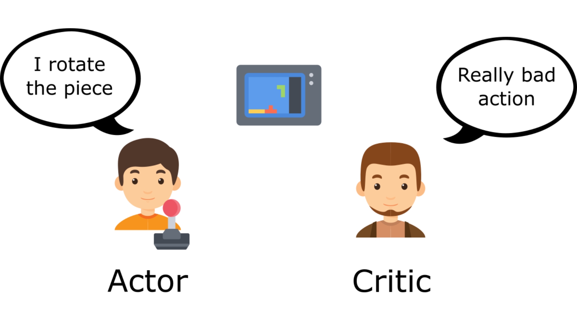
Subtracting the critic's value from the return yields the advantage — how much better an action did than expected — the core of Advantage Actor-Critic (A2C) and of PPO, the workhorse behind much of today's applied RL, including the reinforcement-learning step used to align large language models. Here is how the three families line up:
| Value-based (traditional) | Policy gradient | Actor-critic | |
|---|---|---|---|
| What it learns | Action values Q(s,a) | The policy πθ(a|s) | Both a policy and a value |
| Action spaces | Discrete only | Discrete or continuous | Discrete or continuous |
| Update signal | Low variance, can be biased | Unbiased but high variance | Balanced — critic cuts variance |
| Updates after | Every step | Every episode | Every step |
| Examples | Q-learning, DQN | REINFORCE | A2C, PPO, SAC |
Performance in Dynamic Environments
The tidy assumptions of a gridworld rarely survive contact with reality. Advanced RL is judged by how it copes when the environment stops sitting still.
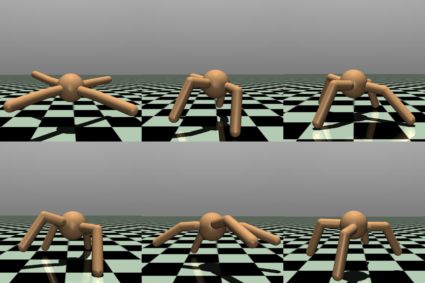
Continuous control is where advanced methods shine and where they are most often benchmarked — physics simulators in which a many-jointed body must learn to move. Gymnasium's MuJoCo suite is the standard testbed.
Because no single algorithm wins everywhere, "performance" in RL is multidimensional. Four axes matter most when evaluating a method:
The through-line from the previous section holds: these are all variations on sensing a state, choosing an action, and adjusting toward a better estimate. What changes at the frontier is how that estimate is represented and stabilized when the world is large, continuous, and refuses to hold still.
Tools & Tutorials
- Hugging Face Deep RL Course — a free, code-first course that walks from DQN through A2C and PPO, with notebooks you train and share; the actor-critic unit pairs directly with this page.
- OpenAI Spinning Up — clear write-ups plus clean, standalone reference implementations of VPG, DDPG, TD3, SAC, and PPO, ideal for reading algorithms end to end.
- Gymnasium MuJoCo environments — runnable continuous-control benchmarks (Ant, HalfCheetah, Humanoid) for testing policy-gradient and actor-critic agents.
Further reading
- Weng, L. (2018). Policy Gradient Algorithms. — a thorough, well-notated tour from REINFORCE through A2C, A3C, DDPG, TRPO, PPO, and SAC; the single best reference for the methods in §2.
- Sutton, R. S. & Barto, A. G. (2018). Reinforcement Learning: An Introduction (2nd ed.). — Chapters 9–13 cover function approximation, policy-gradient methods, and actor-critic in depth.
- Deep Q-Networks (DQN) — A Quick Introduction (with Code). — a concise, code-backed walkthrough of the DQN architecture, experience replay, and target networks introduced in §1.