"Supervised learning is told the right answer. Reinforcement learning is only ever told the score, and has to work backwards from it to figure out what a good decision even was."- Claude 2026
Reinforcement Learning: Fundamentals
Most machine learning is shown a stack of correct answers and asked to imitate them. Reinforcement learning is never shown the answer at all — it acts, receives a score, and has to figure out for itself which decisions were worth making.
Reinforcement learning (RL) is the branch of machine learning concerned with sequential decision-making: an agent interacts with a world over time, and learns a strategy that maximizes a cumulative reward. It is the framework behind game-playing systems that beat human champions, robots that learn to walk, and the fine-tuning step that shapes modern language models. This page builds the vocabulary from scratch — no ML background assumed — then formalizes it as a Markov Decision Process and derives the single most important tabular algorithm, Q-learning, before putting both to work on small problems you can run yourself.
Learning objectives
By the end of this page you should be able to:
- Explain the core concepts of reinforcement learning, including agents, states, and rewards.
- Illustrate the role of Markov Decision Processes and Q-learning in reinforcement learning.
- Apply reinforcement learning algorithms to simple decision-making problems.
The Core Loop: Agent, Environment, Reward
Picture teaching a dog a trick. You never explain the trick in words. The dog tries something, and you either give a treat or you don't. Over many attempts it converges on the behavior that earns treats. Nobody labeled the "correct" muscle movements — the dog inferred them from a stream of rewards. That is reinforcement learning, and it has a precise structure.
The loop above has exactly five moving parts. Everything else in RL is built on them.
One subtlety separates RL from every other kind of learning: rewards are often delayed. A chess move that looks fine may lose the game twenty moves later. The agent therefore cannot just maximize the immediate reward — it must maximize the return, the total reward accumulated from now until the episode ends.
Return, discounting, and the value function
Because a reward now is usually worth more than the same reward far in the future, we weight future rewards by a discount factor γ (gamma), a number between 0 and 1. The return from time t is:
Gt = rt+1 + γ rt+2 + γ2 rt+3 + …
A γ near 0 makes a short-sighted agent that grabs immediate reward; a γ near 1 makes a far-sighted one that plans ahead. The value function V(s) is then the expected return from a state — a forecast of "how good is it to be here?" — and it is what most RL algorithms are really trying to estimate.
Markov Decision Processes and Q-Learning
To reason about the loop mathematically we need one simplifying assumption: the future depends only on the present state, not on the entire history of how we got there. This is the Markov property. A decision problem that satisfies it is a Markov Decision Process (MDP) — the formal object almost all of RL is defined over.
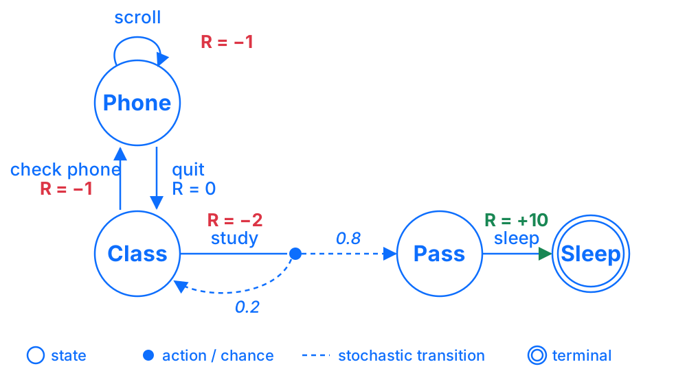
Formally an MDP is a five-part tuple. The diagram above contains every piece of it:
| Symbol | Name | In the student diagram |
|---|---|---|
| S | Set of states | Class, Phone, Pass, Sleep |
| A | Set of actions | study, check phone, scroll, quit, sleep |
| P | Transition probabilities P(s′ | s, a) | study → 0.8 Pass, 0.2 Class |
| R | Reward function | −1 scroll, −2 study, +10 sleep after passing |
| γ | Discount factor | how much future reward counts today |
The Bellman idea: value is recursive
The key insight that makes MDPs solvable is that the value of a state can be written in terms of the value of the states it leads to. Being in a good state means getting a good immediate reward and landing in another good state. This self-referential relationship is the Bellman equation, and every method below is, at heart, a way of turning it into an update rule you can apply repeatedly until the value estimates stop changing.
Q-Learning: learning the value of actions
The Q-learning algorithm learns a Q-value — the quality of taking action a in state s and then behaving optimally afterward. Store these in a table with one row per state and one column per action, and the agent's strategy becomes trivial: in any state, pick the action with the highest Q-value.
The table starts empty (all zeros). After each step the agent nudges one cell toward the reward it just saw plus its current estimate of the best it can do next — the Bellman idea in code:
import numpy as np
q = np.zeros((n_states, n_actions))

def update(q, s, a, r, s_next, alpha=0.1, gamma=0.99):
    best_next = q[s_next].max()
    q[s, a] += alpha * (r + gamma * best_next - q[s, a])
    return q
Here alpha is the learning rate (how big a step to take) and the term in parentheses is the temporal-difference error: the gap between what the agent expected and what actually happened. Repeat this update across enough episodes and the table converges to the optimal action values.
Applying It to Simple Problems
The concepts land fastest on problems small enough to hold in your head. Two are traditional first steps.
The multi-armed bandit: RL stripped to one decision
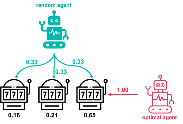
Imagine a row of slot machines ("one-armed bandits"), each paying out at an unknown average rate. You have a fixed number of pulls and want to maximize winnings. There is only one state, so no planning is involved — the entire problem is the exploration–exploitation trade-off in its purest form. Spend too long sampling arms and you waste pulls; commit too early and you may back the wrong machine.
The bandit is the minimal RL problem and the cleanest place to study ε-greedy, optimism, and other action-selection rules before states and transitions complicate the picture.
Gridworld: the first full MDP
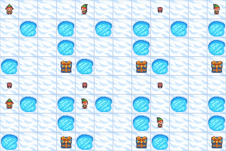
Add states and movement and you get a gridworld: an agent on a grid must reach a goal cell, earning reward there and possibly penalties elsewhere. It is the smallest problem with genuine sequential structure — where an action's worth depends on where it leads several steps later — which is exactly what Q-learning is built to solve.
FrozenLake, shown at right, is the canonical example: cross a frozen grid from start to goal without falling through a hole. In its slippery variant, moves sometimes send you sideways — a built-in stochastic transition function, just like the study MDP earlier.
Putting the loop and the update together, a complete tabular Q-learning agent for FrozenLake is remarkably short. It resets the environment, steps through episodes with an ε-greedy policy, and applies the update from earlier at every step:
import gymnasium as gym
import numpy as np

env = gym.make('FrozenLake-v1', is_slippery=False)
q = np.zeros((env.observation_space.n, env.action_space.n))
alpha, gamma, eps = 0.1, 0.99, 0.1

for episode in range(10000):
    s, _ = env.reset()
    done = False
    while not done:
        explore = np.random.rand() < eps
        a = env.action_space.sample() if explore else int(q[s].argmax())
        s_next, r, terminated, truncated, _ = env.step(a)
        q[s, a] += alpha * (r + gamma * q[s_next].max() - q[s, a])
        s, done = s_next, terminated or truncated
That is the whole idea end to end: sense the state, choose an action (sometimes exploring), observe the reward and next state, and adjust one table entry toward a better estimate. Everything more advanced — function approximation, deep networks, policy gradients — is a way of scaling this same loop to problems too large for a table.
Tools & Tutorials
- REINFORCEjs GridWorld (Karpathy) — an in-browser gridworld where you watch tabular Q-learning and SARSA propagate values in real time; the fastest way to build intuition for what the Q-table is doing.
- Gymnasium — FrozenLake — documentation and a runnable environment for the example above, including the slippery/stochastic variant and the full observation and action spaces.
- Hugging Face Deep RL Course, Unit 2 — a free, hands-on walkthrough that has you implement a Q-learning agent from scratch on FrozenLake, with a Colab notebook and quizzes.
Further reading
- Sutton, R. S. & Barto, A. G. (2018). Reinforcement Learning: An Introduction (2nd ed.). — the definitive textbook; Chapters 3–6 cover MDPs, value functions, and temporal-difference methods including Q-learning.
- Weng, L. (2018). A (Long) Peek into Reinforcement Learning. — a rigorous single-page tour from the agent–environment loop through MDPs, the Bellman equations, and Q-learning, with clean notation.
- Guo, R. et al. (2021). Stochastic inversion of magnetotelluric data using deep reinforcement learning. — a worked application (and the source of the Q-table figure above) showing how the same value-based framework transfers to a real scientific inverse problem.