"A static problem asks you to find the answer. A dynamic one asks you to keep having one."- Claude 2026
Optimization in Dynamic Environments
Almost every optimization method is introduced on a problem that sits perfectly still: a fixed objective, fixed constraints, one best answer waiting to be found. Real problems move while you are solving them. Demand shifts, a machine fails, prices update, the data your model was fitted on stops describing the world. The goal quietly changes from finding an optimum to keeping one — and that change of goal invalidates a surprising amount of standard practice.
Optimization means searching a space of possible answers for the one that scores best under some measure: the objective, a single number to be pushed up or down, subject to constraints that a legal answer must satisfy.

Learning objectives
By the end of this page you should be able to:
- Explain the challenges of optimization in dynamic and uncertain environments.
- Apply AI-driven methods for real-time optimization under changing conditions.
- Assess the adaptability of optimization algorithms in evolving systems.
When the Problem Moves
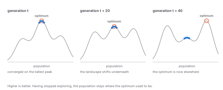
Picture the set of all possible answers as a landscape where height is quality, and optimization as the search for the highest point. In a static problem that landscape is a photograph. In a dynamic problem it is a video: peaks rise and fall, the tallest one moves, and sometimes a region that was legal to stand in becomes off-limits.
Four different things can move, and they demand different responses, so it is worth separating them before choosing a method:
How the change arrives matters as much as what changes. Four shapes recur across the literature, and each suggests a different response:
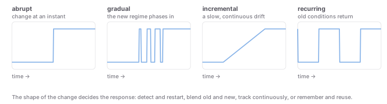
Beyond shape, three properties of the change decide almost every design choice you will make:
| Property | The question | What it decides |
|---|---|---|
| Frequency | How often does the world change relative to how long a solve takes? | Whether you can afford to re-optimize at all, or must run a policy that answers instantly |
| Severity | How far does the optimum move when it moves? | Whether to repair the current solution or start over; small moves reward warm starts, large ones do not |
| Predictability | Is the change forecastable, cyclic, or random? | Whether to anticipate (forecast and pre-position) or merely to react |
| Visibility | Do you get told that something changed? | Whether you need explicit change detection or can simply keep learning continuously |
| Reversibility | Can you undo a committed decision? | How much of the plan to commit to now versus keep open — the value of hedging |
One consequence deserves stating plainly, because it inverts a habit built up on static problems. On a fixed landscape, a population of candidate solutions collapsing onto one answer is success. On a moving landscape it is the loss of the only asset that lets you notice the world has moved. The same is true of a forecasting model that has fit its training data perfectly, and of a solver whose answer is optimal for a snapshot that expired an hour ago.
Methods for Optimizing in Real Time
The practical toolkit divides into five strategies. Most production systems combine several, and the choice between them follows directly from the properties in the table above.
1. Detect the change, then repair rather than restart
If change arrives as discrete events, the first job is noticing. Two mechanisms do this cheaply. Sentinel solutions are a handful of candidates whose scores are re-evaluated every cycle: if a score changes without the candidate changing, the environment did. Statistical drift detectors watch a stream of errors or rewards and signal when its distribution shifts — ADWIN maintains an adaptive window over recent observations and cuts it whenever two sub-windows disagree enough to be unlikely by chance.
Once a change is detected, restarting from scratch is almost always the wrong move. A change of moderate severity leaves most of the previous answer still good, so the efficient response is a warm start: keep the incumbent, repair the parts the change invalidated, and re-optimize locally around it. This is the same destroy-and-repair idea that powers large neighborhood search, applied to time rather than to problem size.
2. Keep diversity on purpose
Population methods such as genetic algorithms and swarm methods lose their ability to react as they converge. Three standard repairs exist, and they can be combined:
- Random immigrants. Replace part of the population with fresh random candidates every generation, or after every detected change, guaranteeing a permanent supply of unexplored ground.
- Hypermutation. Temporarily raise the mutation rate immediately after a change, spraying the population outward, then return it to normal so the search can settle again.
- Multiple populations and memory. Keep sub-populations on different peaks so a rising peak is already occupied when it becomes best, and store good solutions from past environments to re-test when conditions recur.
The effect is easy to measure. Below, five peaks drift every twenty generations; the same genetic algorithm runs with and without random immigrants plus a short burst of hypermutation after each change. The score reported is tracking error — how far the best solution found since the last change falls short of the true optimum, averaged over every generation:
import math
import random

random.seed(3)
span, dim, n_peaks = 50.0, 2, 5
peaks = [[random.uniform(0, span) for _ in range(dim)] for _ in range(n_peaks)]
heights = [random.uniform(40, 70) for _ in range(n_peaks)]

def score(x):
    return max(h - 0.8 * math.dist(x, c) for c, h in zip(peaks, heights))

def shift(severity=6.0):
    for c in peaks:
        for i in range(dim):
            c[i] = min(span, max(0.0, c[i] + random.gauss(0, severity)))

def random_point():
    return [random.uniform(0, span) for _ in range(dim)]

def run(adaptive, generations=300, interval=20, size=30):
    random.seed(11)
    pop = [random_point() for _ in range(size)]
    trace, best_since_change, age = [], None, 0
    for g in range(generations):
        if g and g % interval == 0:
            shift()
            best_since_change, age = None, 0
            if adaptive:
                pop[size // 2:] = [random_point() for _ in range(size - size // 2)]
        sigma = 6.0 if adaptive and age < 3 else 1.0
        pop.sort(key=score, reverse=True)
        best = score(pop[0])
        best_since_change = best if best_since_change is None else max(best_since_change, best)
        trace.append(max(heights) - best_since_change)
        parents = pop[:size // 3]
        pop = [p[:] for p in parents]
        while len(pop) < size:
            a, b = random.sample(parents, 2)
            child = [(u + v) / 2 + random.gauss(0, sigma) for u, v in zip(a, b)]
            pop.append([min(span, max(0.0, v)) for v in child])
        age += 1
    return trace

converged = run(adaptive=False)
adaptive = run(adaptive=True)
print('converged GA', round(sum(converged) / len(converged), 2))
print('adaptive GA ', round(sum(adaptive) / len(adaptive), 2))
The converged run averages a tracking error of 1.33; the adaptive one, 0.43 — the same algorithm, the same budget, three times closer to the moving optimum. Plotting the error generation by generation shows why, and it is not that the adaptive run is generally better:
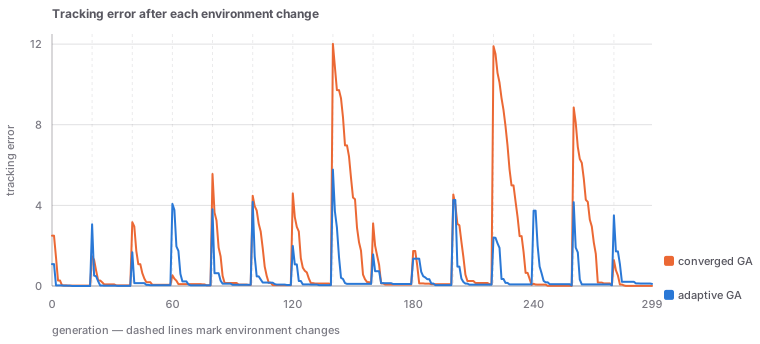
The advantage also grows with severity, which is the honest way to report this kind of result — a single number hides the fact that diversity mechanisms cost you nothing much when changes are tiny and save you everything when they are large:
| Change severity | Converged GA | Adaptive GA | Ratio |
|---|---|---|---|
| 6 | 1.33 | 0.43 | 3.1× |
| 10 | 2.69 | 0.52 | 5.2× |
| 15 | 4.72 | 0.59 | 8.0× |
3. Predict, commit once, re-plan
Where a forecast exists, the dominant industrial pattern is model predictive control (MPC), also called receding-horizon control. At each step, use a model to predict how the system will evolve, optimize a whole sequence of decisions over that horizon, then throw away all but the first decision, take a fresh measurement, and solve again.
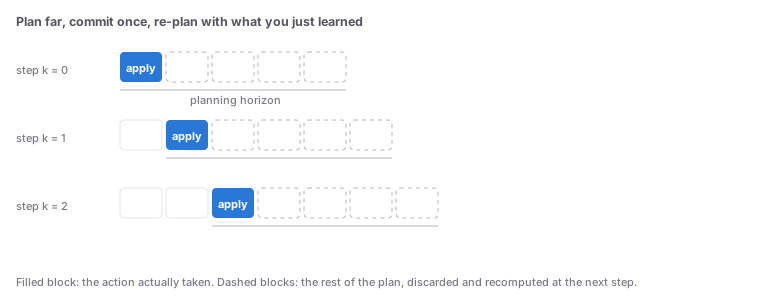
MPC is how a building pre-cools before a hot afternoon, how a battery decides when to charge against a price forecast, and how a chemical plant holds a setpoint through disturbances. It also inherits the weakness of its model: when the forecast is biased, the plan is confidently wrong, which is why MPC is usually paired with feedback that corrects the model as measurements arrive.
4. Learn online — and forget on purpose
When no usable model of the environment exists, the alternative is to learn a decision rule directly from outcomes. In a changing world the natural measure of success is not "did we find the optimum" but regret: how much worse did the decisions we actually made do, compared with the best decisions available in hindsight? Regret is defined over a sequence, which is exactly the right shape for a problem that never ends.
The smallest instructive case is the multi-armed bandit: several options with unknown payoffs, one choice per round, and only the chosen option's payoff observed. The non-stationary version adds the twist that the payoffs drift over time. There, the classic estimator — average all rewards ever seen for each option — becomes actively harmful, because every stale observation gets equal weight forever. Replacing it with a constant step size makes the estimate an exponentially weighted average of recent rewards, so old evidence decays away:
import numpy as np
rng = np.random.default_rng(0)

arms, steps, runs, epsilon = 10, 10000, 50, 0.1

def testbed(alpha=None):
    reward = optimal = 0
    for _ in range(runs):
        true_value = np.zeros(arms)
        estimate, count = np.zeros(arms), np.zeros(arms)
        for _ in range(steps):
            a = rng.integers(arms) if rng.random() < epsilon else int(estimate.argmax())
            r = rng.normal(true_value[a], 1.0)
            count[a] += 1
            estimate[a] += (alpha or 1 / count[a]) * (r - estimate[a])
            reward += r
            optimal += a == int(true_value.argmax())
            true_value += rng.normal(0, 0.01, arms)
    total = runs * steps
    return reward / total, 100 * optimal / total

for name, alpha in (('sample average', None), ('constant step ', 0.1)):
    r, pct = testbed(alpha)
    print(f'{name}  reward {r:5.2f}  optimal {pct:4.1f}%')
The averaging rule earns 0.69 per step and picks the genuinely best option 43.9% of the time; the forgetting rule earns 0.91 and picks it 67.1% of the time. Nothing about the search changed — only how much the past is allowed to count. Every method in this section is, in some form, a decision about that.
5. When you cannot react, be robust
Some decisions are committed before the uncertainty resolves and cannot be revised: where to build the depot, which contracts to sign, what to load on the truck before it leaves. Here the answer is not a faster loop but a different objective. Robust optimization asks for the plan whose worst case across a set of plausible futures is best; stochastic optimization asks for the plan with the best expected outcome across those futures. Both deliberately give up peak performance on the future that actually happens, in exchange for not collapsing on the ones that might.
The same idea appears in learned controllers as domain randomization: train across many randomized variations of the environment so the resulting policy does not depend on any one of them being accurate.
The constraints that only exist in real time
Three requirements have no equivalent in static optimization, and they routinely decide which method is usable:
Assessing Adaptability
The standard report for a static optimizer — the quality of the final answer — is meaningless here, because there is no final answer. A dynamic optimizer is judged on a whole trajectory, and the useful measures capture different failures:
| Measure | What it is | The failure it catches |
|---|---|---|
| Tracking (offline) error | Average gap to the true optimum over every time step | Sustained mediocrity, including between changes |
| Recovery time | Steps needed to return within a threshold of the optimum after a change | A method that is excellent when settled and helpless when disturbed |
| Regret | Cumulative shortfall against the best decisions in hindsight | Slow learning and over-exploration, on problems with no defined "optimum" |
| Worst-case error | The largest gap reached at any point | Rare but unacceptable excursions hidden by a good average |
| Stability / churn | How much the solution changes per cycle | A plan too volatile to execute in the real world |
| Cost of adaptation | Compute, data and evaluations spent per change | Adaptivity bought at a price exceeding the loss it avoids |
Because these must be measured against a known moving target, the field relies on generators rather than fixed instances. The Moving Peaks Benchmark — the setting the code in §2 imitates — generates a landscape whose peaks shift in position, height and width at a controlled frequency and severity, so the optimum is known at every instant. Dynamic variants of routing and scheduling problems add customers or machine failures mid-solve, and drifting data streams do the same for learned components.
Interrogating an adaptive-optimization claim
One more caution, familiar from every applied setting: a method tuned on a particular drift pattern has, in effect, been told what will happen. If the tuning set contains only gradual drift, expect the method to fail on the abrupt change that eventually arrives — the dynamic-environment version of overfitting.
Two Systems That Cannot Pause
Controlling a fusion plasma. The image at the top of this page shows plasma inside the Tokamak à Configuration Variable at EPFL's Swiss Plasma Center. Plasma is held in place by magnetic fields produced by control coils, and it is unstable: the state evolves continuously and a wrong command is unrecoverable within milliseconds. Conventional practice engineers a separate controller for each desired plasma shape, a slow and specialised process. Researchers instead trained a reinforcement learning agent in simulation to map measurements directly to coil voltages, then deployed the trained network inside the tokamak's real-time control loop, where it produced and held a range of plasma configurations — including elongated shapes and a configuration with two separate plasmas held simultaneously (Degrave et al., Nature, 2022). It is the clearest demonstration that a learned policy can meet a hard real-time deadline in a genuinely unforgiving environment — and also a clear illustration of the cost: the simulator, the safety analysis, and the engineering around the policy dwarf the policy itself.
Retiming traffic signals from observed traffic. Traffic is dynamic on every timescale — hour, day, season, roadworks — while signal timing plans are typically set once and left for years. Google's Project Green Light models intersections from aggregated Maps driving trends, identifies where the timing no longer matches the traffic, and hands city engineers recommendations they can implement on existing hardware.
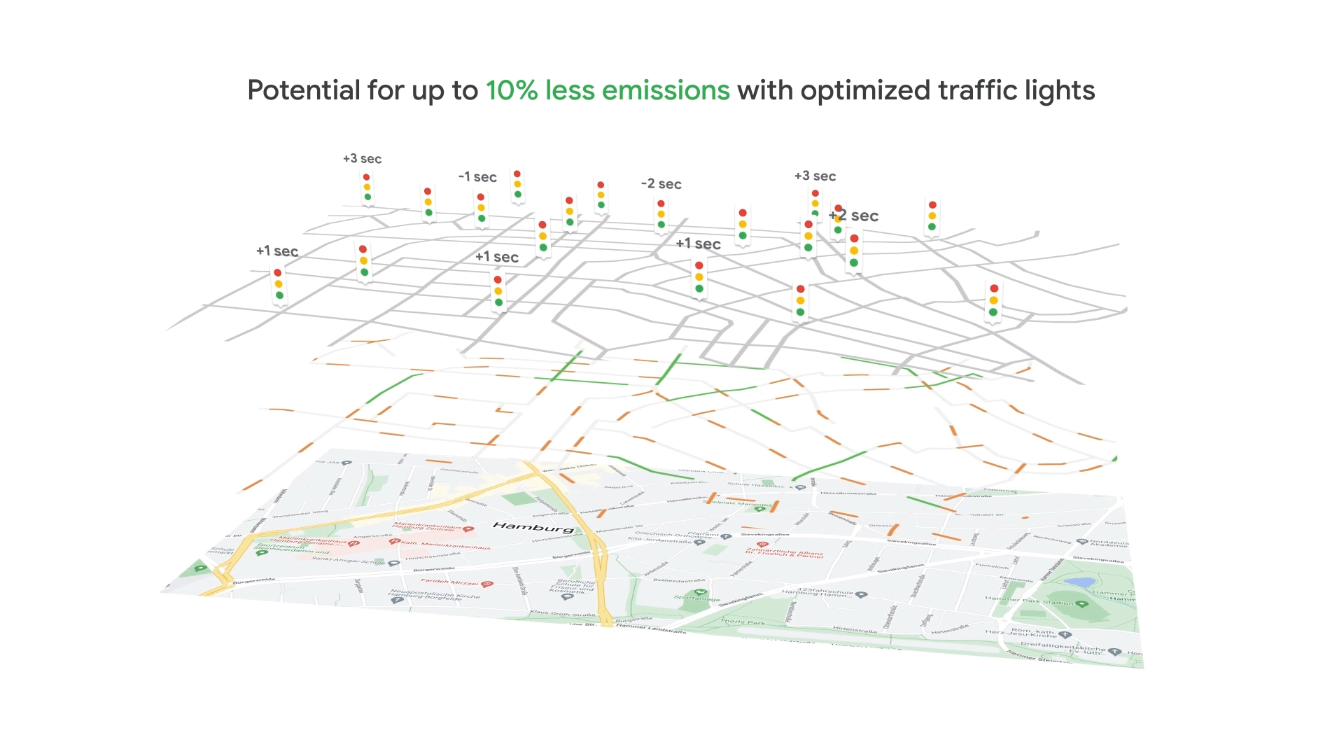
The two sit at opposite ends of a spectrum worth noticing. The plasma controller closes the loop in milliseconds with no human in it; Green Light closes the loop in weeks with a city engineer in the middle, and gets its adaptivity from re-solving as observations accumulate rather than from any online algorithm. Both are optimization in a dynamic environment. The difference is only how fast the environment moves relative to how fast a decision can be made and acted on — which is, in the end, the single number that organizes this whole subject.
Tools & Tutorials
- River — concept drift detection — a short, runnable walkthrough that generates a drifting stream and detects the change points with ADWIN; the rest of the library is built for models that learn one observation at a time.
- do-mpc — an open-source Python toolbox for model predictive control and moving-horizon estimation, with getting-started tutorials and a gallery of worked closed-loop examples including robust multi-stage MPC.
- Vowpal Wabbit — contextual bandit content personalization — a notebook-style tutorial that simulates a recommender and then swaps the reward function halfway through, so you can watch a learner recover from a change of preferences.
- Eclipse SUMO — TraCI traffic light tutorial — control signals from a Python script that reads live detector state inside a running traffic simulation: a small, complete closed loop you can modify.
- EDOLAB — an open-source MATLAB platform bundling 25 dynamic-optimization algorithms and three benchmark generators (including the Moving Peaks Benchmark), with animated visualisation of how the landscape changes between environments.
Further reading
- Yazdani, D., Cheng, R., Yazdani, D., Branke, J., Jin, Y. & Yao, X. (2021). A survey of evolutionary continuous dynamic optimization over two decades — Part A. IEEE Transactions on Evolutionary Computation, 25(4). — the standard reference for the problem definitions, benchmark generators and performance measures used in §3; free accepted manuscript.
- Lu, J., Liu, A., Dong, F., Gu, F., Gama, J. & Zhang, G. (2020). Learning under Concept Drift: A Review. — over 130 papers organised into detection, understanding and adaptation, plus the synthetic and real benchmark datasets the area evaluates on.
- Hazan, E. (2023). Introduction to Online Convex Optimization (2nd ed.). — the theory behind treating optimization as a never-ending sequence of decisions, and where regret bounds come from.
- Lattimore, T. & Szepesvári, C. (2020). Bandit Algorithms. Cambridge University Press. — free full text; Chapter 31 covers non-stationary bandits, the formal version of the forgetting experiment in §2.
- Degrave, J. et al. (2022). Magnetic control of tokamak plasmas through deep reinforcement learning. Nature, 602, 414–419. — the full account of the plasma-control case study, including the simulation-to-hardware transfer and the real-time constraints it had to meet.
- Kirkpatrick, J. et al. (2017). Overcoming catastrophic forgetting in neural networks. — why continuously updated models lose old competence, and one influential remedy.