"Every resource decision is the same question wearing different clothes: limited supply, competing demands, and a number you are trying to make as large or as small as you can."- Claude 2026
AI-Driven Optimization in Resource Management
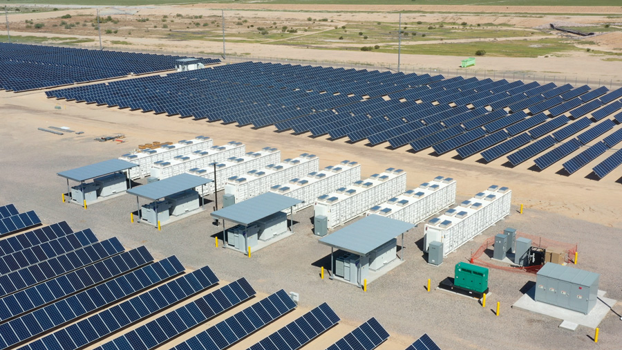
A resource is anything there is not enough of: megawatts, cardboard, machine hours, water, memory, money, staff. Resource management asks two questions about all of them — who or what gets each unit, and how much useful work comes out of it. Both are optimization questions, and both are now routinely answered by algorithms operating at a speed and scale no planning department could match.
Learning objectives
By the end of this page you should be able to:
- Explain strategies for resource allocation and utilization using AI optimization.
- Apply optimization algorithms to improve the efficiency of energy and material resources.
- Assess the impact of AI-driven optimization on sustainability and cost reduction.
Allocation, Utilization, and the Shape of the Problem
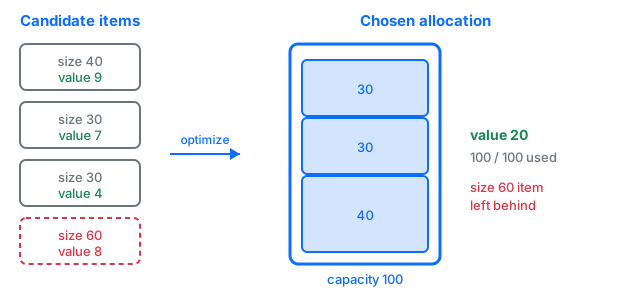
Allocation is the assignment decision: which generator serves which demand, which item goes in which box, which job runs on which machine. Utilization is the efficiency question that follows: of the capacity you committed, how much did real work, and how much was idle, wasted, or spilled. A plant running at 40% of capacity and a half-empty shipping container are the same failure in different units.
Nearly every resource problem collapses into one of a small set of classical templates. Recognizing which one you have is most of the work, because each template comes with known algorithms:
| Template | The question it asks | Resource example | Typical method |
|---|---|---|---|
| Knapsack | Which subset of items maximizes value within one capacity limit? | Which projects to fund from a fixed budget | Dynamic programming, integer programming |
| Bin packing | How few containers can hold everything? | Cartons, trucks, servers in a rack | Heuristics, constraint programming |
| Assignment | Which agent should be matched to which task? | Crews to shifts, jobs to machines | Hungarian algorithm, min-cost flow |
| Linear programming | How much of each continuous resource to use? | Megawatts per plant, tonnes per supplier | Simplex, interior point |
| Scheduling | What happens when, given precedence and capacity? | Maintenance windows, batch production | Constraint programming, metaheuristics |
Strategies for Allocation and Utilization
Three axes separate one resource-management approach from another. Getting them right matters more than the choice of any particular algorithm.
Static vs. dynamic
A static plan is computed once for a known situation — next quarter's supplier contracts. A dynamic or online policy decides continuously as information arrives: dispatching power minute by minute, admitting jobs to a cluster as they queue. Dynamic problems reward methods that can decide fast and revise, not methods that need an hour of solve time.
Centralized vs. distributed
One optimizer with a global view produces the best plan when it can see everything. When resources are owned by many parties, or the network is too large to model centrally, control is distributed: local agents follow simple rules and coordinate through prices or signals. Distributed control sacrifices optimality to gain robustness and scale.
Solved vs. learned
A solver computes the answer from an explicit model of the world. A learned policy is trained on data or simulation and outputs decisions directly. Solvers are auditable and constraint-respecting; learned policies handle messiness the model omits. Production systems increasingly use both.
Within the "solved vs. learned" axis sits the pragmatic middle ground that most industrial systems occupy — predict, then optimize. A machine learning model forecasts the uncertain quantities (tomorrow's demand, wind output, failure risk), and a classical optimizer takes those forecasts as inputs and produces a plan that provably satisfies the constraints. The forecast absorbs the uncertainty; the solver guarantees the plan is legal.
When the environment is too complex to model explicitly, the field reaches for search and learning methods that need only a way to score a candidate:
Energy Resources
Electricity is the hardest resource to manage because it must be produced and consumed in the same instant, and because the cheapest sources are now the least controllable. The core allocation problem — economic dispatch — asks how much each generator should produce right now to meet demand at minimum cost, subject to capacity limits and, increasingly, an emissions ceiling.
This is a linear program, and it is small enough to write out completely. Four plants with different marginal costs and carbon intensities must cover 120 MW of demand while staying under a carbon cap:
import pulp

plants = {'solar': (0, 40), 'wind': (2, 30), 'gas': (55, 80), 'coal': (35, 60)}
carbon = {'solar': 0, 'wind': 0, 'gas': 0.45, 'coal': 0.95}
demand, carbon_cap = 120, 40

model = pulp.LpProblem('dispatch', pulp.LpMinimize)
out = {p: pulp.LpVariable(p, 0, cap) for p, (_, cap) in plants.items()}

model += pulp.lpSum(cost * out[p] for p, (cost, _) in plants.items())
model += pulp.lpSum(out.values()) == demand
model += pulp.lpSum(carbon[p] * out[p] for p in plants) <= carbon_cap

model.solve(pulp.PULP_CBC_CMD(msg=False))
for p in plants:
    print(f'{p:6s} {out[p].value():6.1f} MW')
print(f'cost   {pulp.value(model.objective):6.1f}')
The solver returns solar 40, wind 30, gas 15, coal 35 — total cost 2110. Note what the carbon cap did: coal is cheaper per megawatt than gas, so a purely cost-minimizing run would have burned far more of it. The constraint binds exactly at 40 units of carbon, and the model buys the last 15 MW from the more expensive but cleaner plant. That single line is the entire mechanism by which a policy target becomes an operational decision.
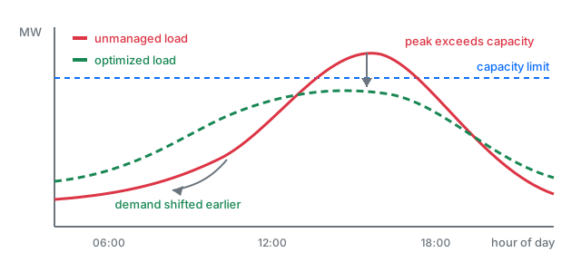
Real grids extend this in every direction — hundreds of units, start-up costs and minimum run times (the unit commitment problem), transmission limits, storage, and demand forecasts that are themselves model outputs. Two ideas do most of the work on the demand side:
Case study: learning to cool a data centre
Data centre cooling is a control problem with dozens of interacting knobs — pumps, chillers, cooling towers, heat exchangers — whose optimal settings depend on load, outside weather, and each other. Google trained neural networks on years of sensor data to predict future power usage effectiveness (PUE, the ratio of total facility energy to IT energy) from candidate control settings, then used those models to choose settings.
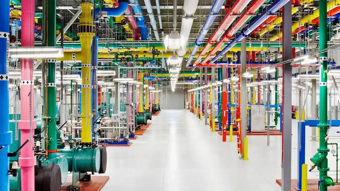
The follow-up system moved from recommendations to direct autonomous control, and its architecture is the template for safe learned control of physical resources: the AI proposes actions, a verification layer checks them against hard safety constraints, local plant controllers can reject anything unsafe, and operators can take over at any moment. The intelligence is allowed to optimize only inside a box drawn by conventional engineering.
Material Resources
Material efficiency has three levers: use less per unit, waste less in processing, and invent better materials outright. AI now works on all three.
Use less per unit. Amazon's Package Decision Engine chooses the packaging for each item — box, padded mailer, paper bag, or no extra packaging at all — from computer vision measurements at intake, text about the product, and damage signals from returns and reviews. The system reportedly cut packaging weight per shipment substantially and avoided millions of tonnes of material, work that previously depended on physically testing products one at a time and could never have scaled to hundreds of millions of items.
Waste less in processing. Cutting stock and packing decide how much raw material becomes product and how much becomes offcut. Here is the bin-packing template solved exactly with a constraint solver — ten items, containers of capacity 100, minimizing containers used:
from ortools.sat.python import cp_model

sizes = [48, 30, 19, 36, 36, 27, 42, 42, 36, 24]
capacity, max_bins = 100, 5

model = cp_model.CpModel()
x = {(i, b): model.new_bool_var(f'x{i}_{b}') for i in range(len(sizes)) for b in range(max_bins)}
used = [model.new_bool_var(f'u{b}') for b in range(max_bins)]

for i in range(len(sizes)):
    model.add_exactly_one(x[i, b] for b in range(max_bins))
for b in range(max_bins):
    model.add(sum(sizes[i] * x[i, b] for i in range(len(sizes))) <= capacity * used[b])

model.minimize(sum(used))
solver = cp_model.CpSolver()
solver.solve(model)

for b in range(max_bins):
    packed = [sizes[i] for i in range(len(sizes)) if solver.value(x[i, b])]
    if packed:
        print(f'bin {b}: {packed} -> {sum(packed)}/{capacity}')
Total demand is 340 units, so no solution can use fewer than four containers, and the solver finds a four-container packing. Scale this up — thousands of items, real geometry, weight limits, fragility rules — and exact methods give way to heuristics and learned packing policies, but the objective never changes: fewer containers, fuller containers, less air shipped.
Invent better materials. The most upstream intervention is to find materials that need less of a scarce element in the first place. Graph neural networks trained on known crystal structures can predict the stability of hypothetical compounds far faster than physical simulation, turning materials discovery into a search problem over a combinatorial space of candidate structures.

Assessing Sustainability and Cost Impact
Claimed savings are the least reliable numbers in this field. A percentage without a baseline, a pilot that ran during a mild summer, an "AI-optimized" system that also came with new hardware — all of these produce impressive figures that mean very little. Assessing impact honestly requires asking the same questions every time.
Interrogating a resource-optimization claim
Two structural effects deserve attention beyond the arithmetic. The first is the rebound effect, or Jevons paradox: making a resource cheaper to use tends to increase how much of it gets used. Efficiency gains that lower unit cost can be partly or wholly consumed by expanded demand, so efficiency alone is not a decarbonization strategy — it needs a cap or a price to bind against, exactly like the carbon constraint in the dispatch model above.
The second is that AI is itself a resource consumer. Training and serving large models draws electricity, water for cooling, and materials for hardware. A resource-optimization project should be able to state, at least roughly, that the resources it saves exceed the resources it spends — and the systems with the best case here are typically the unglamorous ones: a small forecasting model plus a classical solver, running on modest hardware, saving megawatts.
Tools & Tutorials
- PuLP — the Python linear programming library used in the dispatch example; its case studies work through blending, scheduling and allocation models from scratch.
- OR-Tools knapsack guide — a runnable walkthrough of the single-capacity selection problem, the simplest resource allocation model there is.
- OR-Tools bin packing guide — the container-minimization problem behind the second code example, including the multiple-knapsack variant.
- CityLearn — an open simulation environment for training and benchmarking control policies on building energy, storage and demand response; a practical way to experiment with learned energy control without a building.
- PyPSA — open-source Python toolbox for modelling and optimizing power systems, including dispatch, storage and network investment on realistic grids.
- Electricity Maps data portal — free hourly carbon-intensity data by region: the input signal any carbon-aware scheduler needs.
Further reading
- Google DeepMind (2016). DeepMind AI reduces Google data centre cooling bill by 40%. — the original account of the learned cooling controller and the on/off experiment behind this page's chart.
- Google DeepMind (2018). Safety-first AI for autonomous data centre cooling and industrial control. — how the recommendation system became a direct controller, and the layered safety architecture that made it acceptable.
- Radovanović, A. et al. (2021). Carbon-Aware Computing for Datacenters. — the design and production results of Google's system for shifting flexible compute toward low-carbon hours.
- Merchant, A. et al. (2023). Scaling deep learning for materials discovery, Nature. — the peer-reviewed paper behind the crystal structure search, including how candidates were generated and filtered.
- Amazon (2024). How Amazon is using AI to deliver customer orders with less packaging. — first-hand description of the Package Decision Engine's inputs, decisions and reported material savings.
- Green Software Foundation. — specifications and patterns for measuring and reducing the energy and carbon cost of software itself, including the Software Carbon Intensity standard.