The Role of Randomness in Algorithm Design
Why Randomness Helps
A deterministic algorithm produces the same output on every run for the same input. An adversary who knows the algorithm can construct inputs that trigger worst-case behaviour — a sorted array fed to a naïve QuickSort, for example, yields O(n²) time. A randomized algorithm receives, in addition to its input, a stream of random bits it uses to make choices. This denies the adversary any fixed “bad input”: the worst case depends on the random bits, which the adversary cannot control.
Three ways randomness helps:
1. Breaking adversarial structure — random pivot selection prevents sorted input from being worst-case for QuickSort.
2. Simpler algorithms — Karger's random min-cut is far simpler than the best deterministic min-cut algorithm, yet achieves comparable complexity.
3. Problems with no known deterministic solution — before 2002, no polynomial-time deterministic primality test was known; Miller–Rabin's randomized test was the practical standard for decades.
Monte Carlo vs. Las Vegas — The Fundamental Distinction
Las Vegas in Practice: Randomized QuickSort
Breaking the Adversary with a Random Pivot
Deterministic QuickSort selects a fixed pivot (e.g. the last element). On a sorted array, every partition produces one element and n−1 elements, giving O(n²) comparisons — worst-case performance an adversary can always trigger. Randomized QuickSort simply selects the pivot uniformly at random.
Expected time analysis: Define an indicator variable Xij = 1 if element i and element j are ever compared. By linearity of expectation, E[comparisons] = ∑ Pr[Xij = 1]. Elements i and j are compared only if one of them is chosen as a pivot before any element strictly between them in sorted order. The probability of this is 2/(j−i+1). Summing over all pairs: E[comparisons] = O(n log n) — independent of the input.
The key insight: The randomness defeats any adversary. No matter what input is given, the expected runtime is O(n log n). The algorithm never fails — it always produces a correctly sorted array — making it Las Vegas. With high probability (probability at least 1 − 1/n), the actual runtime is O(n log n), not just in expectation.
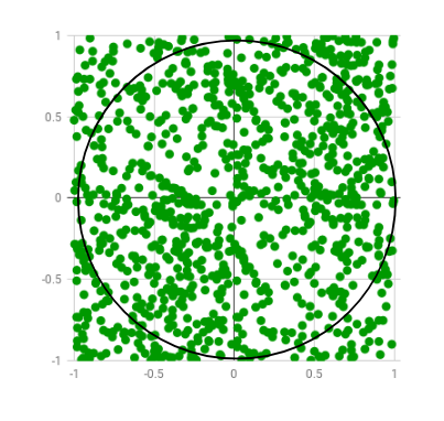
Monte Carlo in Practice: Estimating π by Sampling
Miller–Rabin Primality Testing — Monte Carlo at Scale
The problem: Given a large integer n, determine whether it is prime. Naïve trial division runs in O(√n) time — exponential in the number of bits of n. Before 2002, no deterministic polynomial-time test was known.
Fermat's little theorem: If n is prime, then for any a not divisible by n, an−1 ≡ 1 (mod n). Miller–Rabin tests this condition with additional structure (the Rabin witness) for a randomly chosen base a. If n is composite, at least 3/4 of all possible bases are witnesses to its compositeness.
The algorithm: Choose k random bases a1, ..., ak. If any base detects compositeness, return “composite” (definitely). If all bases pass, return “probably prime.” The probability of error is at most (1/4)k — less than one in a trillion for k = 20. Runtime: O(k log² n). This is the algorithm RSA key generation uses in practice.
Comparison with Las Vegas: Miller–Rabin is Monte Carlo — it may (very rarely) declare a composite number prime. AKS (2002) is a deterministic O((log n)6) primality test — but Miller–Rabin is faster in practice for cryptographic key sizes (512–4096 bits) and the error probability is negligibly small.
Karger's Algorithm — Randomized Graph Theory
Karger's Algorithm — Minimum Cut by Random Contraction
The problem: Given an undirected graph G = (V, E), find a minimum cut — a partition of V into two non-empty sets S and V\S minimising the number of edges crossing the partition. Minimum cut has important applications in network reliability, image segmentation, and clustering.
The algorithm: While more than 2 vertices remain, select an edge (u, v) uniformly at random, contract it (merge u and v into a single vertex, keeping parallel edges but removing self-loops), and repeat. Return the remaining edges between the two vertices as the cut.
Analysis: If the minimum cut has k edges, the probability that a single run finds it is at least 2/(n(n−1)) ≈ 2/n². By running the algorithm O(n² log n) times and taking the best cut found, the probability of missing the minimum cut is at most 1/n. Total time: O(n´ log n). This is polynomial — and for sparse graphs, randomized approaches outperform deterministic ones.
Randomized Techniques — Applied Problems
Randomized Complexity Classes
ZPP (Zero-Error Poly-Time)
The class of Las Vegas algorithms: always correct, expected polynomial runtime. Formally, ZPP = RP ∩ co-RP. Problems in ZPP include primality testing (after 2002, AKS places it in P; before, Miller–Rabin suggested it was in ZPP ∩ BPP). P ⊆ ZPP ⊆ RP ⊆ NP.
RP (Randomized Poly-Time)
Decision problems solvable with a polynomial-time randomized algorithm that never errs on NO-instances and succeeds on YES-instances with probability ≥ 1/2. One-sided error. Pr[false positive] = 0; Pr[false negative] ≤ 1/2. Repeat k times to reduce error to 2−k.
BPP (Bounded-Error Poly-Time)
The randomized analogue of P: decision problems solvable with polynomial-time Monte Carlo algorithms with error probability ≤ 1/3 on all inputs. Two-sided error. Most cryptographers believe BPP = P (derandomization conjecture), though this is unproven. P ⊆ BPP.
Derandomization
The goal of removing randomness while preserving performance. A pseudorandom generator (PRG) produces a stream indistinguishable from true randomness for any efficient algorithm. If strong PRGs exist, BPP = P. Nisan–Wigderson (1994) showed hardness implies derandomization.
Resources & Further Reading