The Complexity Class Hierarchy
Computational complexity classifies decision problems by the resources — time, space, nondeterminism — required to solve or verify them. The four classes P, NP, NP-complete, and NP-hard form a hierarchy that captures the most practically important distinctions in all of theoretical computer science.
P is the class of decision problems solvable by a deterministic Turing machine in time O(nk) for some constant k. Problems in P are considered tractable: we possess algorithms whose running time scales manageably with input size. Sorting (O(n log n)), shortest path (Dijkstra, O(n²)), linear programming (polynomial via interior point methods), and primality testing (AKS, O(n6)) are all in P.
NP is the class of decision problems for which a "yes" answer has a polynomial-size certificate (witness) that can be verified in polynomial time by a deterministic TM. Equivalently, NP is the class of problems decidable in polynomial time by a nondeterministic TM. Note that P ⊆ NP: any problem solvable in polynomial time is trivially verifiable in polynomial time (the computation trace itself is the certificate).
A problem H is NP-hard if every problem in NP can be polynomial-time reduced to H. Formally: for all L ∈ NP, L ≤p H. NP-hard problems are at least as hard as the hardest problems in NP. Crucially, an NP-hard problem need not itself be in NP — it may not even be decidable. The Halting Problem is NP-hard (everything reduces to it) but is undecidable and hence not in NP.
A problem X is NP-complete if it satisfies two conditions: (1) X ∈ NP, and (2) X is NP-hard. NP-complete problems are precisely the hardest problems in NP. They sit at the intersection of NP and NP-hard. A polynomial-time algorithm for any single NP-complete problem would immediately yield polynomial-time algorithms for every problem in NP — collapsing the hierarchy so that P = NP.
- In P but trivially also in NP: Sorting, shortest path, 2-SAT, matching in bipartite graphs. Solvable and verifiable in polynomial time.
- In NP, believed not in P: 3-SAT, Hamiltonian Cycle, Graph Colouring (k ≥ 3), Subset Sum. Solutions are easy to verify but no polynomial-time algorithm is known for finding them.
- NP-complete: All of the above "believed not in P" examples. They are in NP and every NP problem reduces to them.
- NP-hard but not in NP: The Halting Problem, the optimisation version of TSP ("find the shortest tour" — the answer is a number, not a yes/no). These are at least as hard as NP-complete problems but cannot be efficiently verified (or are not even decision problems).

Image: Wikimedia Commons, CC BY-SA 3.0
Polynomial-Time Reductions and NP-Completeness Proofs
The mechanism that connects NP-complete problems to one another — and that allows us to prove new problems NP-complete — is the polynomial-time reduction. The idea is deceptively simple: if you can transform instances of problem A into instances of problem B in polynomial time such that answers are preserved, then B is at least as hard as A.
A Karp reduction from language A to language B is a polynomial-time computable function f: Σ* → Σ* such that for all strings w: w ∈ A ⟺ f(w) ∈ B. We write A ≤p B. If A ≤p B and B ∈ P, then A ∈ P. Contrapositively: if A is hard, then B must be at least as hard.
The Cook-Levin Theorem: The First NP-Completeness Proof
Every NP-completeness proof ultimately traces back to a single foundational result: the Cook-Levin theorem (Cook, 1971; Levin, 1973). This theorem establishes that SAT is NP-complete by showing that the computation of any nondeterministic polynomial-time Turing machine can be encoded as a Boolean formula — so that the formula is satisfiable if and only if the machine accepts.
- Goal: Show that for any L ∈ NP, L ≤p SAT.
- Setup: Since L ∈ NP, there exists a nondeterministic TM M that decides L in time nk. The computation of M on input w can be represented as an nk × nk tableau: each row is a configuration (tape contents + head position + state).
- Encoding: Introduce Boolean variables for each cell of the tableau. Construct clauses ensuring: (1) each cell contains exactly one symbol, (2) the first row encodes the start configuration on w, (3) consecutive rows follow M's transition function, and (4) some row contains an accept state.
- Result: The formula φ is satisfiable ⟺ M accepts w ⟺ w ∈ L. The construction runs in polynomial time (O(n2k) variables and clauses). Therefore L ≤p SAT.
Reduction Chains: Karp's 21 Problems
Once SAT is known to be NP-complete, proving new problems NP-complete becomes much easier: you only need to show a reduction from a known NP-complete problem to the new candidate (plus membership in NP). In 1972, Richard Karp demonstrated this strategy by reducing SAT to 21 important combinatorial problems — establishing all of them as NP-complete through a chain of reductions.
- Input: A 3-CNF formula φ with m clauses over n variables.
- Construction: For each clause (l1 ∨ l2 ∨ l3), create a triangle gadget of three vertices (one per literal) with edges between all three. Then add edges between every pair of vertices whose labels are complementary (xi and ¬xi).
- Claim: φ is satisfiable ⟺ the constructed graph has an independent set of size m.
- Why it works: An independent set of size m must pick exactly one vertex from each triangle (selecting a true literal per clause). The complementarity edges prevent picking both xi and ¬xi, ensuring the selection corresponds to a consistent truth assignment.
- Conclusion: Since 3-SAT is NP-complete and 3-SAT ≤p Independent Set, Independent Set is NP-hard. Since Independent Set ∈ NP (a proposed set is trivially verified), it is NP-complete.
Step 1: Show X ∈ NP — exhibit a polynomial-time verifier (given an instance and a certificate, the verifier checks correctness in polynomial time). Step 2: Choose a known NP-complete problem Y and construct a polynomial-time reduction Y ≤p X. This proves X is NP-hard. Steps 1 and 2 together give NP-completeness. The art lies in choosing Y wisely and designing "gadgets" that faithfully encode Y-instances as X-instances.
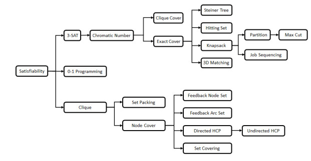
Image: Source
The P vs NP Question
The central question is: does P = NP? In concrete terms: if every problem whose solutions can be checked in polynomial time can also be solved in polynomial time, the classes collapse. If not — if there exist problems in NP that provably require super-polynomial time — then P ≠ NP and the hierarchy stands.
Most researchers believe P ≠ NP. A 2019 survey of complexity theorists found that 88% believe P ≠ NP, about 9% are unsure, and fewer than 3% believe P = NP. But belief is not proof. The question was designated one of the seven Clay Millennium Prize Problems in 2000, carrying a $1,000,000 prize, and remains open.
- If P = NP: Every problem whose answer can be verified quickly can also be solved quickly. Polynomial-time algorithms would exist for SAT, graph colouring, TSP, scheduling, protein folding, and thousands of other NP-complete problems. RSA and elliptic curve cryptography would be broken (factoring and ECDLP are in NP). Mathematical theorem proving could in principle be automated. The practical implications would be revolutionary — or catastrophic, depending on one's perspective.
- If P ≠ NP: There are fundamentally hard problems whose solutions we can recognise but not efficiently discover. Cryptography rests on firm theoretical ground. Algorithm designers are justified in seeking approximations and heuristics rather than exact polynomial-time solutions for NP-hard problems. The universe has inherent computational asymmetry between creation and verification.
Implications for Algorithm Design
The P vs NP question is not merely philosophical — it directly governs the strategies that algorithm designers use in practice. When a problem is shown to be NP-complete, the response is not to give up but to shift strategy.
Coping with NP-Hardness
Once a problem is identified as NP-hard, exact polynomial-time algorithms are believed impossible. Practitioners instead rely on several well-developed strategies, each with distinct trade-offs.
- Approximation algorithms: Find solutions provably within a constant factor of optimal in polynomial time. For example, the greedy algorithm for Vertex Cover achieves a 2-approximation. The Christofides-Serdyukov algorithm for metric TSP guarantees a 3/2-approximation.
- Parameterised complexity (FPT): Isolate a parameter k (e.g., solution size) and find algorithms running in f(k) · nc time, where f is exponential in k but c is constant. Vertex Cover is FPT: solvable in O(2k · n) time. If k is small, this is practical even for large n.
- Heuristics and metaheuristics: Use greedy methods, local search, simulated annealing, or genetic algorithms. No worst-case guarantee, but often effective in practice. SAT solvers using DPLL and conflict-driven clause learning (CDCL) routinely solve industrial instances with millions of variables.
- Special-case tractability: Restrict the problem structure. 2-SAT is in P (while 3-SAT is NP-complete). Planar graph colouring with 4 colours is always possible (Four Colour Theorem). Tree-structured constraint satisfaction problems are polynomial.
- Randomised algorithms: Allow a small probability of error or use expected polynomial time. Randomised rounding of linear programming relaxations is a powerful technique for NP-hard optimisation problems.
Reductions as a Design Tool
Reductions are not only a proof technique — they are a practical tool. If you can reduce your problem to SAT, you can use a highly optimised SAT solver as a "universal NP engine." Modern SAT solvers, despite the worst-case exponential bound, solve structured instances extraordinarily fast due to decades of engineering. This approach — encode your problem as SAT (or Integer Linear Programming, or Constraint Satisfaction), then apply an off-the-shelf solver — is one of the most powerful strategies in practical algorithm design.
- Cryptography: The security of RSA depends on integer factorisation being hard (factorisation is in NP ∩ co-NP but not known to be NP-complete). If P = NP, all public-key cryptography based on NP-hard assumptions collapses. Even if P ≠ NP, this does not prove specific cryptographic assumptions — it only means that hard problems exist somewhere in NP.
- Machine learning: Many learning problems (training optimal neural networks, feature selection) are NP-hard. In practice, gradient descent and stochastic methods work well despite worst-case intractability — suggesting that real-world instances have exploitable structure.
- Operations research: Scheduling, vehicle routing, facility location, and network design are NP-hard. Industry relies on approximation algorithms, mixed-integer programming solvers, and heuristic search — all strategies motivated by the belief that exact polynomial-time solutions do not exist.
- Verification and formal methods: Model checking and satisfiability testing are NP-hard in general but solvable in practice for structured instances. The gap between worst-case theory and average-case practice is enormous — and understanding this gap is an active research area.
Beyond P and NP: The Broader Landscape
P and NP anchor a much richer hierarchy. co-NP contains problems whose "no" instances have short certificates (e.g., "this formula is unsatisfiable" — the complement of SAT). PSPACE captures problems solvable in polynomial space, containing both NP and co-NP. BPP (bounded-error probabilistic polynomial time) captures efficiently solvable problems with randomisation. EXPTIME contains problems requiring exponential time — and we do know P ⊊ EXPTIME (a rare strict separation). Whether NP ⊆ P, NP ⊆ BPP, or NP ⊆ PSPACE are strict containments remains, in each case, open.