Space Complexity and Its Classification
Time complexity asks how many steps an algorithm takes; space complexity asks how much memory it needs. These two resources are related but distinct — some problems can be solved in polynomial time but require enormous space, while others need very little space but exponential time. Understanding space complexity reveals structural properties of computation that time alone cannot capture.
SPACE(f(n)) is the class of decision problems solvable by a deterministic Turing machine using at most O(f(n)) cells of work tape (beyond the read-only input tape). NSPACE(f(n)) is the analogous class for nondeterministic Turing machines. Space is measured on a separate work tape so that sub-linear space classes (using less memory than the input size) are meaningful.
L (or LOGSPACE) = SPACE(log n): problems solvable using only logarithmic space. A machine with O(log n) work tape can store a constant number of pointers into the input — enough to traverse a graph but not enough to store it. NL = NSPACE(log n): problems solvable nondeterministically in logarithmic space. The canonical NL-complete problem is PATH (st-connectivity): given a directed graph G and vertices s, t, is there a path from s to t?
PSPACE = ∪k≥1 SPACE(nk): problems solvable in polynomial space. PSPACE contains both P and NP (since a polynomial-time computation uses at most polynomial space). The canonical PSPACE-complete problem is TQBF (True Quantified Boolean Formulas): given a fully quantified Boolean formula ∀x₁∃x₂∀x₃…φ, determine whether it is true. TQBF generalises SAT by adding universal quantifiers, making it harder — it captures alternating computation and game-like reasoning.
Fundamental Theorems of Space Complexity
Several landmark theorems reveal the deep structure of space-bounded computation and connect space classes to time classes in surprising ways.
- Savitch's Theorem (1970): NSPACE(f(n)) ⊆ SPACE(f(n)²) for f(n) ≥ log n. Nondeterminism gives at most a quadratic blowup in space — dramatically less than the exponential gap believed to separate P and NP in time. In particular, NL ⊆ SPACE(log² n) and NPSPACE = PSPACE.
- Immerman–Szelepcsényi Theorem (1987): NSPACE(f(n)) = co-NSPACE(f(n)) for f(n) ≥ log n. Nondeterministic space classes are closed under complement. This means NL = co-NL — a result with no known analogue in time complexity (whether NP = co-NP remains open).
- Space Hierarchy Theorem: For space-constructible f and g with f(n) = o(g(n)), SPACE(f(n)) ⊊ SPACE(g(n)). More space strictly means more power — there exist problems solvable in O(n²) space that cannot be solved in O(n) space.
- PSPACE ⊆ EXPTIME: Any polynomial-space computation has at most exponentially many distinct configurations, so it halts in exponential time. Combined with the Time Hierarchy Theorem (P ⊊ EXPTIME), this gives us L ⊆ NL ⊆ P ⊆ NP ⊆ PSPACE ⊆ EXPTIME, with P ≠ EXPTIME being one of the few known strict separations.
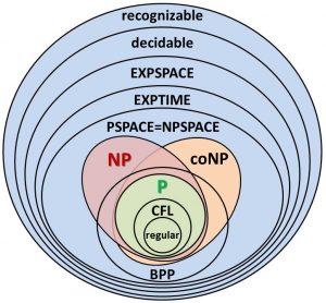
Image: Source
Probabilistic Complexity Classes
Classical complexity theory assumes deterministic or nondeterministic computation. But what happens when an algorithm can flip fair coins? Randomness introduces a powerful new resource — one that appears to help in practice (randomised algorithms are often simpler and faster than their deterministic counterparts) but whose theoretical power remains one of the great open questions.
BPP is the class of decision problems solvable by a probabilistic polynomial-time Turing machine with error probability at most 1/3 on any input. The error can be reduced to 2−n by repeating and taking a majority vote (polynomial repetitions suffice). BPP is the "practical" probabilistic class — problems in BPP are efficiently solvable with high confidence. It is known that P ⊆ BPP ⊆ PSPACE, but whether P = BPP is a major open question. Many complexity theorists believe P = BPP — that randomness does not actually help.
RP (Randomised Polynomial time) is the class of problems where the algorithm always rejects "no" instances and accepts "yes" instances with probability ≥ 1/2. Errors are one-sided: false negatives are possible, false positives are not. co-RP is the complement: false positives are possible, false negatives are not. The relationship is P ⊆ RP ⊆ BPP and P ⊆ co-RP ⊆ BPP. Polynomial identity testing (Schwartz-Zippel) is a classic example in co-RP.
ZPP = RP ∩ co-RP. A ZPP algorithm always gives the correct answer but its running time is a random variable with polynomial expectation. ZPP is also called "Las Vegas" complexity — the algorithm may be lucky or unlucky in speed but never wrong. Randomised quicksort is a classic ZPP algorithm (expected O(n log n), always correct).
- P ⊆ ZPP ⊆ RP ⊆ BPP: Deterministic is a special case of zero-error random, which is a special case of one-sided error, which is a special case of two-sided error.
- BPP ⊆ P/poly: BPP can be simulated by polynomial-size circuits (Adleman's theorem). This suggests randomness may not provide super-polynomial speedup.
- If strong pseudorandom generators exist, then P = BPP: Under plausible hardness assumptions (e.g., E requires exponential circuits), every BPP algorithm can be efficiently derandomised. This conditional result is why many believe P = BPP.
- BPP vs NP: The relationship is unknown. BPP is not known to contain NP or vice versa. If NP ⊆ BPP, the polynomial hierarchy collapses (Sipser-Lautemann), which is considered unlikely.
Interactive Proofs and IP = PSPACE
Randomness becomes especially powerful when combined with interaction. An interactive proof system involves a computationally unbounded prover and a probabilistic polynomial-time verifier exchanging messages. The verifier must accept valid proofs with high probability and reject invalid ones with high probability.
IP is the class of problems possessing interactive proof systems with a polynomial-time probabilistic verifier. The landmark Shamir's Theorem (1992) proved that IP = PSPACE. This was stunning: it showed that a polynomial-time verifier with randomness and interaction can verify any computation that a polynomial-space machine can perform — far beyond what a static NP certificate can capture.
- Recall that NP captures problems with static polynomial-size certificates. IP allows multi-round dialogue — the verifier can ask adaptive questions.
- Graph Non-Isomorphism is in IP but not known to be in NP. The verifier uses randomness to challenge the prover in ways that a deterministic verifier cannot.
- The proof that IP = PSPACE uses arithmetisation: converting Boolean formulas into polynomials over finite fields and using the Schwartz-Zippel lemma to verify evaluations.
- IP = PSPACE implies that the power of polynomial-space computation can be "checked" by a resource-limited but interactive and randomised agent.
Case Studies: Problems Requiring Advanced Complexity Models
Some problems resist classification within the simple P/NP framework and require the richer machinery of space complexity, probabilistic classes, or interactive proofs. These case studies illustrate why the full complexity landscape matters.
Case Study 1: Primality Testing — From RP to P
- The problem: Given an integer n, is it prime?
- Classical status: Primality was long believed to require randomness. The Miller-Rabin test (1976/1980) placed PRIMES in co-RP — it can certify compositeness with certainty but only certify primality probabilistically.
- Breakthrough: In 2002, Agrawal, Kayal, and Saxena (AKS) gave a deterministic polynomial-time algorithm, proving PRIMES ∈ P. This confirmed the long-held suspicion but required novel algebraic techniques.
- Significance: PRIMES demonstrates that randomness was not necessary — the problem migrated from co-RP to P. It provides evidence (though not proof) for the conjecture P = BPP.
Case Study 2: Quantified Boolean Formulas — PSPACE-Completeness
- The problem: Given a fully quantified Boolean formula ∀x₁∃x₂∀x₃…∃xₙ φ(x₁,…,xₙ), is the formula true?
- Complexity: TQBF is PSPACE-complete. Unlike SAT (which has only existential quantifiers), TQBF involves alternation between universal and existential quantification — modelling adversarial scenarios where one player picks variables to make the formula true and the other tries to falsify it.
- Applications: TQBF captures two-player game evaluation (who has a winning strategy in chess, Go, or generalised Hex?), AI planning with adversarial uncertainty, and formal verification of reactive systems. These problems are inherently harder than NP-complete problems — they require reasoning about all possible opponent moves, not just finding one satisfying assignment.
- Why NP is insufficient: A SAT certificate is a single assignment. A TQBF "certificate" would need to describe a strategy tree — exponentially large in general. This is why TQBF (and game-playing problems) escape NP and land in PSPACE.
Case Study 3: Graph Isomorphism — Between P and NP-Complete
- The problem: Given two graphs G and H, is there a bijection between their vertex sets that preserves adjacency?
- Complexity status: Graph Isomorphism (GI) is in NP (a permutation mapping serves as a certificate). It is not known to be in P and is not known to be NP-complete. It is one of very few natural problems in NP that resist classification into either camp.
- Babai's breakthrough (2015): László Babai showed that GI can be solved in quasi-polynomial time: 2O((log n)³). This places GI tantalisingly close to P — far below the exponential barrier but not quite polynomial.
- Structural reasons: GI is in co-AM (a probabilistic class), and if GI were NP-complete, the polynomial hierarchy would collapse (Boppana-Håstad-Zachos). This structural evidence strongly suggests GI is not NP-complete — making it a rare natural problem in the "twilight zone" between P and NP-complete.
- Connection to space/randomness: The complement problem (Graph Non-Isomorphism) has an interactive proof but no known short static certificate — it lives naturally in IP rather than NP. This makes GI a showpiece for why classes beyond P and NP are essential.
Case Study 4: Stochastic Satisfiability — Merging Randomness and Quantification
- The problem: Stochastic SAT (SSAT) extends TQBF by adding randomised quantifiers alongside ∀ and ∃. A randomised quantifier assigns a variable uniformly at random. The question: is there a strategy achieving probability ≥ θ of satisfaction?
- Complexity: SSAT is complete for PSPACE. It naturally models decision-making under uncertainty: an agent (∃) acts, nature (random quantifier) introduces uncertainty, an adversary (∀) opposes — interleaved across multiple rounds.
- Applications: Probabilistic planning in AI, Markov decision processes with adversarial components, and stochastic game solving all reduce to SSAT. These problems require reasoning about space, probability, and adversarial choice simultaneously — none of the simpler classes (P, NP, BPP) suffice.
The Broader Complexity Landscape
Space complexity, probabilistic computation, and interactive proofs represent just three axes of a vast complexity-theoretic landscape. Other important directions include circuit complexity (measuring the size or depth of Boolean circuits), communication complexity (how much information must be exchanged between parties to compute a function), quantum complexity (what problems quantum computers can solve efficiently — the class BQP), and counting complexity (how hard is it to count solutions, not just find one — the class #P). Each axis reveals different facets of computational hardness and has distinct connections to practical computing.
The overarching lesson is that computational difficulty is not a single spectrum from "easy" to "hard." Problems can be easy in time but hard in space, easy with randomness but hard without it, easy to verify interactively but impossible to verify statically. The richness of complexity theory lies in mapping these distinctions — and in the deep, often surprising connections between seemingly unrelated models of computation.